
Every magnetometer calibration guide says the same thing: tumble the unit in all directions. It sounds like the one easy step. Pick it up, turn it every way you can think of, put it down.
I did that, a lot, starting in February. I pointed the unit in what felt like every direction there is and got calibrations that were mediocre, or good on paper and bad in the water. There’s still a file in my tools folder called mag_baseline_samples 2pct RMS but bad headings.csv. I named it that in April, when I knew it was true and had no idea why.
Part of the fix was tooling. Calibrating used to mean downloading files to a laptop and transferring files back and forth, and now it doesn’t. But the bigger problem was that I didn’t know what good calibration data looked like, and nothing I’d built could show me. Most of this post is screens that showed me something that looked like an answer and wasn’t.
What’s being calibrated
The compass is a three-axis magnetometer. Everything near it adds a small magnetic field of its own: the circuit board, the battery, the motor, the steel in the scooter. Calibration measures those fields and subtracts them, in three steps:
- Baseline. The unit comes off the scooter and gets tumbled through every orientation. (More on “every orientation” in a moment.) This corrects the sensor and its own board, as well as the unit’s own battery, any ferrous material in the housing, and so on.
- Mounted. Back on the scooter, to correct for the motor, battery and hull.
- Heading. Twelve known bearings, one every 30°. Whatever error is left gets fitted as a smooth curve and subtracted.
Post #1 covers why this is where all the accuracy lives.
The baseline needs every orientation because the fit is rebuilding a sphere. Each reading is a point: the direction and strength of Earth’s field as the sensor sees it. A perfect sensor puts every point on a sphere centred on zero. A real one puts them on a squashed sphere sitting off-centre, and the fit works out how squashed and how far off. Show it only part of the sphere and it will happily fit something that matches the part it saw.
The baseline calibration is also just the unit, not the scooter. It’s pretty much impossible to rotate a full-size DPV through “every orientation.” But we still need to know what the impact of the scooter’s magnetics are. So the compromise is two separate calibration collections.
The screens that looked like answers
Coverage: 100%
The first calibration screen had a countdown and two bars.
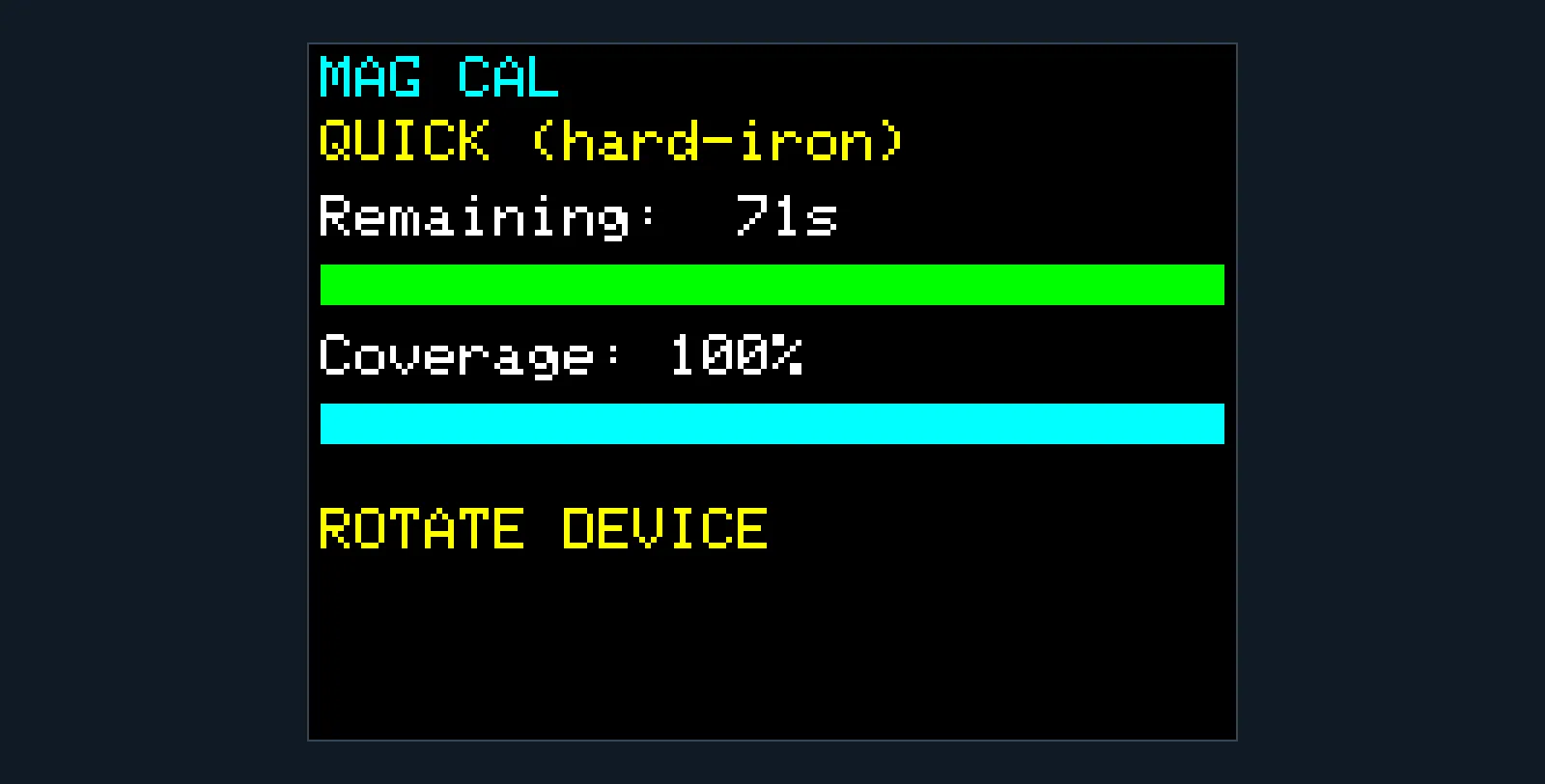
“Coverage” was the spread between the largest and smallest reading on each axis, averaged over the three. A few flicks of the wrist max it out while missing most of the sphere. It would happily say 100% with more than a minute still on the clock. The indication I was showing — time and coverage — had no bearing on whether the math would produce good calibration results.
A grid that went green
By April the unit had a proper coverage grid: 12 headings across, 5 elevation bands down, and each box filling red, then yellow, then green as samples landed in it. It was very satisfying to watch. It also couldn’t be trusted, for a reason that took me until July to see. The grid sorted samples by the unit’s own heading, and heading needs a calibrated compass. That’s the thing the grid was helping to collect. During a baseline, the heading it was sorting by was little better than a wild guess.
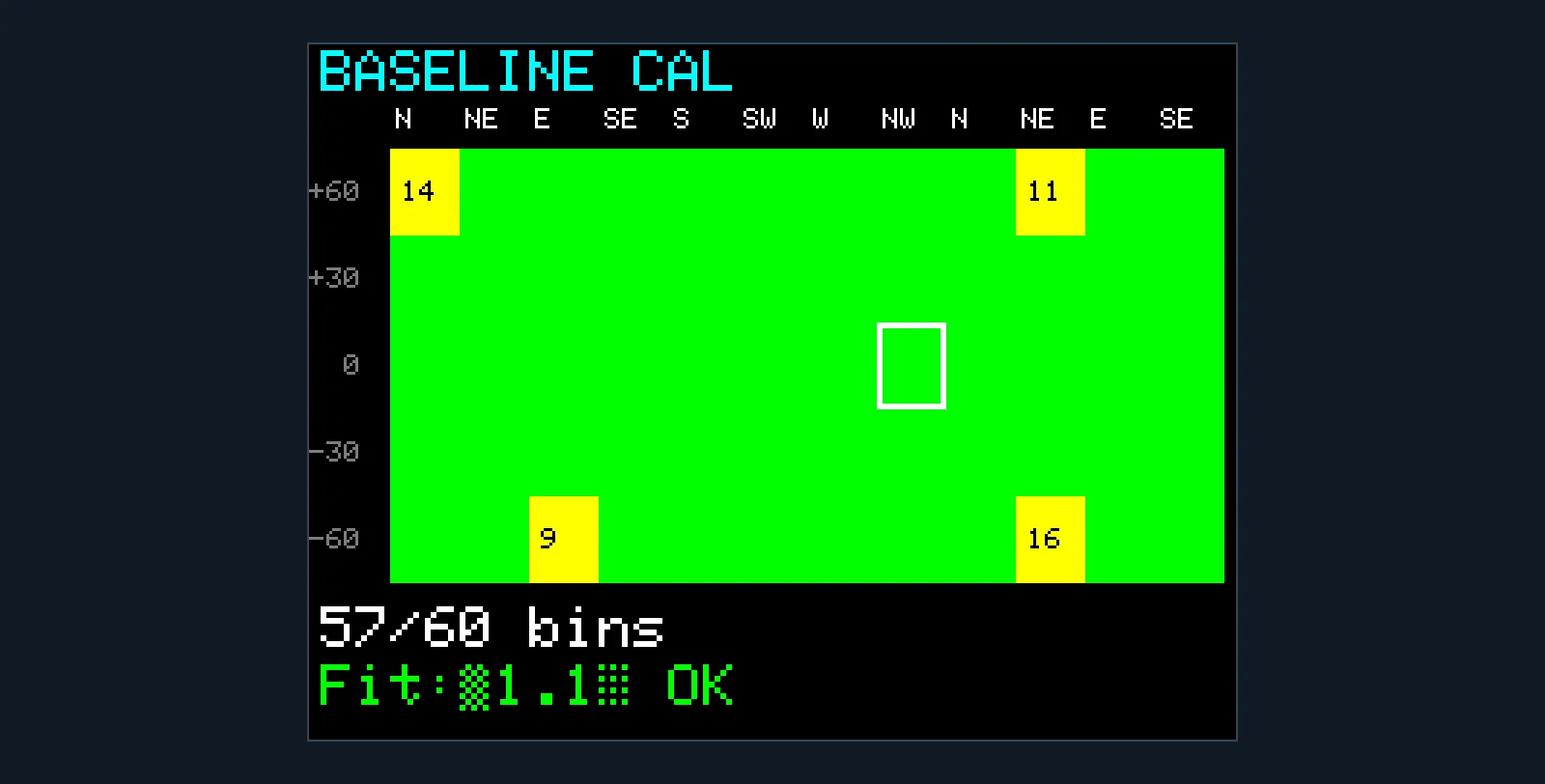
The “Fit ±1.1° OK” line was a live estimate of heading error. It worked that out from how round the fitted circle was, which made it blind to the circle sitting off-centre, and off-centre is the error that matters most. “OK” meant the number had stopped changing, not that it was right.
GOOD (<2% RMS)
Then the samples went to the laptop.
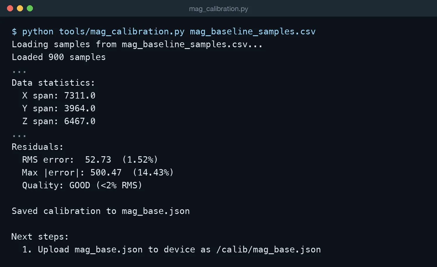
The script printed one number, RMS: on average, how far the corrected samples sit from a perfect sphere. Under 2% was GOOD. Look at the spans, though. The Y axis covered barely half the range of X, because the tumble had missed a big slice of orientations. The fit matched the samples it had beautifully. RMS can only grade the samples you collected. It has no way to see the ones you didn’t.
The laptop errand
A full calibration meant doing this three times, once per step:
- Run the cal on the unit. The samples land in a CSV on its flash.
- Download the CSV from the unit’s web page.
- Run a Python script on the laptop.
- Upload the resulting JSON back to the unit, with exactly the right filename.
- Unplug the battery and plug it back in again (no power switch in those days!)
The heading step’s done screen just listed the homework.
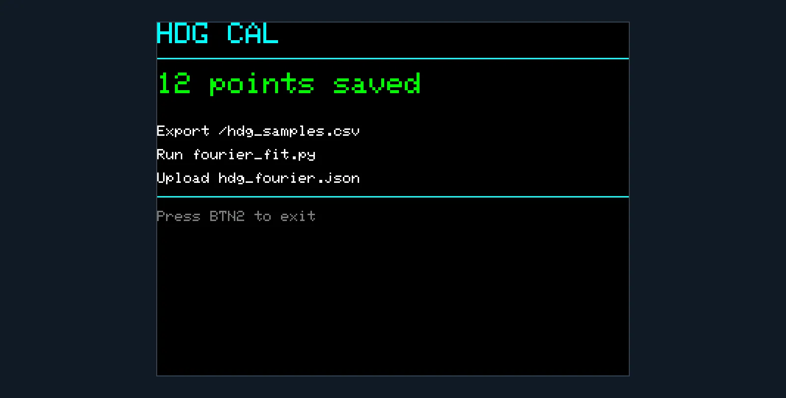
Every manual step was another chance for a correct fit to become a wrong installed calibration. The results also lived in whatever folder I’d run the script from, so there was no history and no good way to compare two attempts.
The curve that hit every point
The heading step had its own version of the same trap.
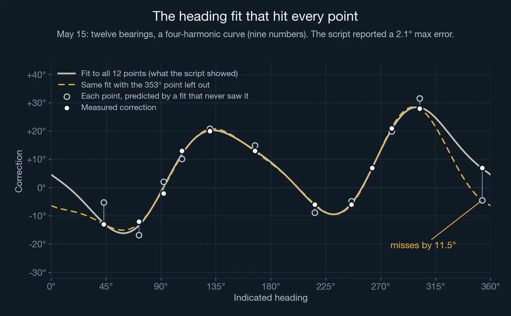
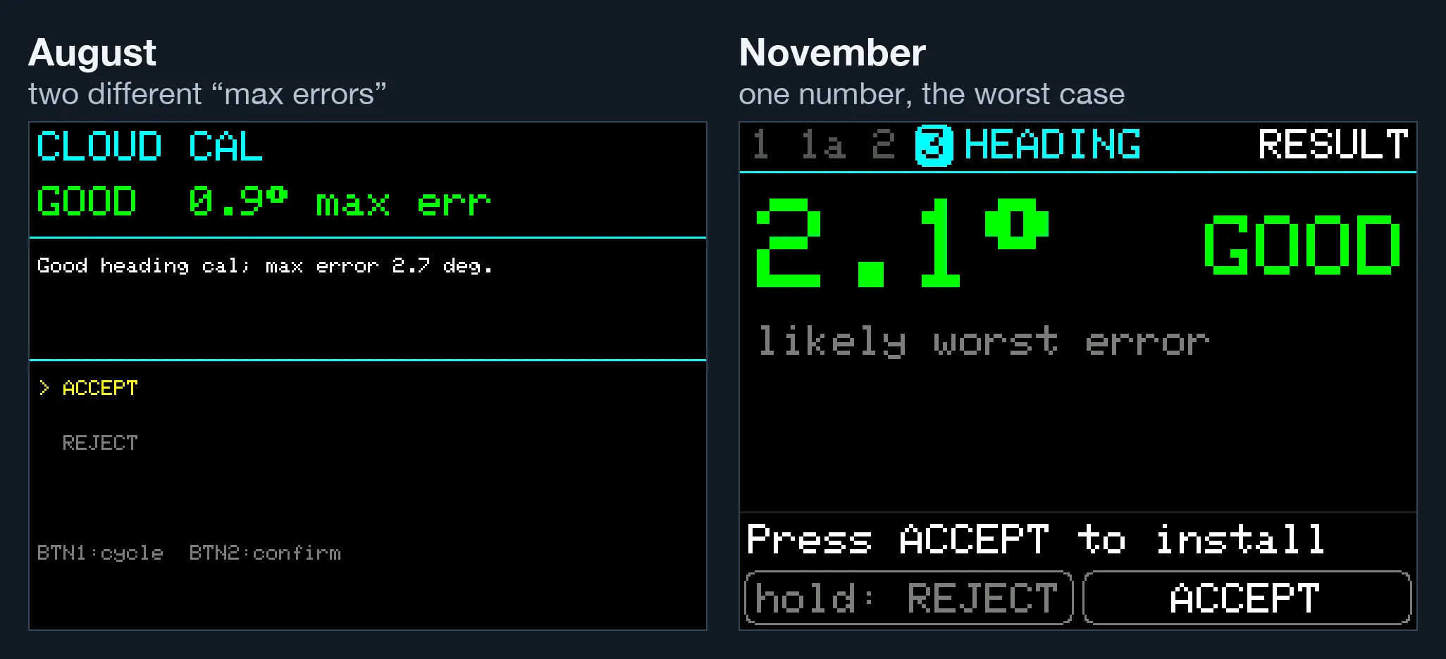
The script tried one to four harmonics and kept adding them until the max error dropped under 3°. Four harmonics is nine numbers, and nine numbers through twelve points will go through nearly all of them. It reported a 2.1° max error, and the four-harmonic curve is what it saved.
The honest test is to hold each point out, fit the other eleven, and see how badly the curve misses the one it never saw. For this fit, the worst miss is 11.5°. It goes wrong in the gaps, between 302° and 353° and between 167° and 216°, where no points were holding it down. Since August the heading fit keeps at least six spare points, which caps a 12-point run at two harmonics. Since October, the number on the result screen is that held-out worst case.
Why it hurt: I didn’t know what good data looked like
The laptop was the pain I could see. The real problem was that I didn’t know what I was trying to collect.
“All directions” sounds obvious. Here’s what it actually produced.
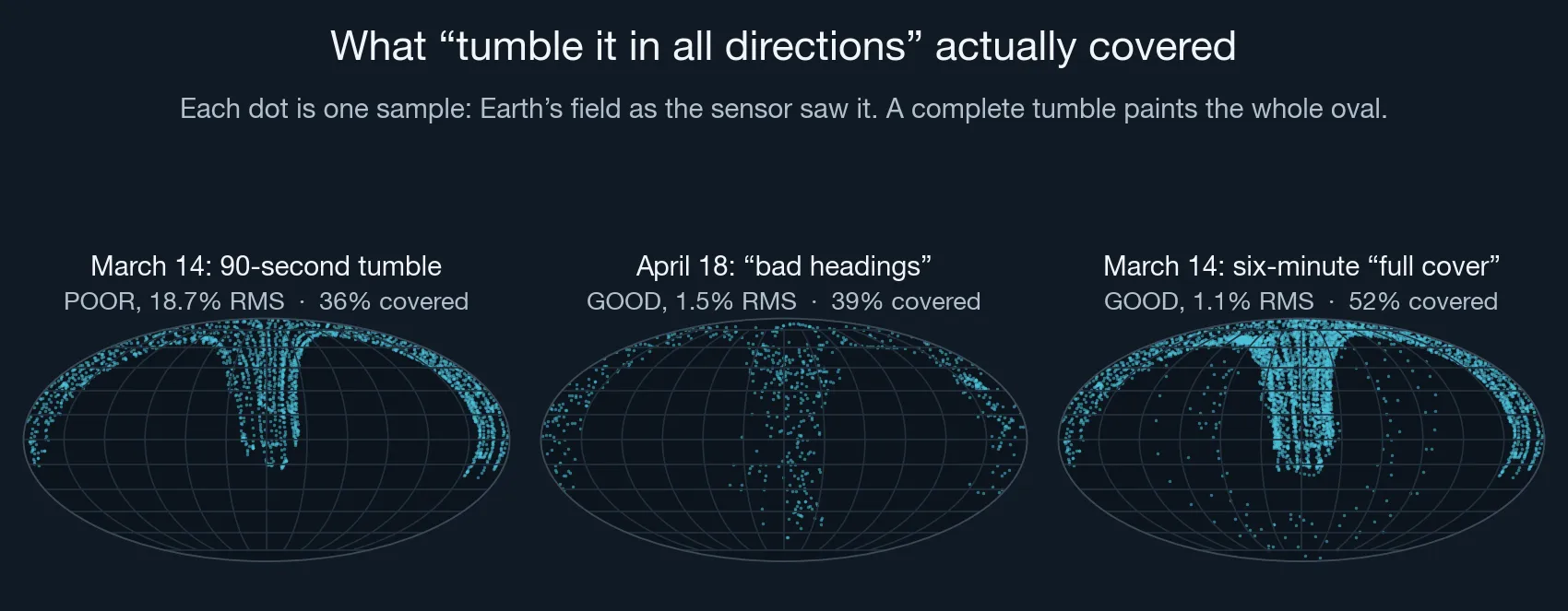
Each dot is one sample: the direction of Earth’s field as the sensor saw it, flattened like a map of the globe. A complete tumble would paint the whole oval. The 90-second tumble covers about a third of it. The six-minute run I’d named “full cover” still left about a quarter of the sphere with nothing in it. And the April run I later labelled “bad headings” scored GOOD with half the sphere empty.
That’s the whole problem in one picture. My hands went where hands go. They covered the comfortable orientations over and over and barely touched the rest, and I had no way to see it. Every tool I had was either blind to the gaps, or, like the grid, claimed to see them using a heading it didn’t actually have.
Six ways not to draw a grid
In July I tried to fix the feedback on the unit itself. There were six attempts, all failed, and all for the same reason underneath: you can’t show someone which way they’ve been pointing until you know where north is, and finding north is what the calibration is for.
- The heading grid above, sorting samples by a heading that was close to a guess.
- A lattice of 60 evenly spaced points on the sphere, which doesn’t need a heading at all. On hardware, the highlight jumped around for no visible reason. The lattice spaces its points evenly by deliberately scattering consecutive numbers around the sphere, so points that are neighbours in space don’t land in neighbouring boxes on screen.
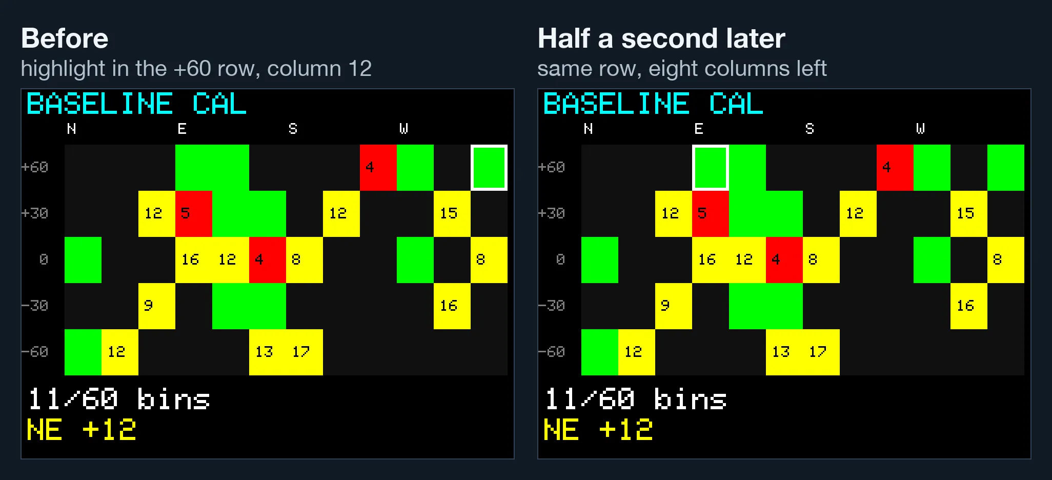
- A grid around a fixed sensor axis. Pointing the unit up filled the bottom boxes, because the axis was wherever Earth’s field happened to point relative to the chip. Worse, the contortions needed to satisfy that display produced a worse calibration than just tumbling naturally.
- Two passes: a rough scan to estimate the offset, then the grid. On hardware, there was still no relationship between how I held the unit and which box lit up.
- One bar per axis. These can all read 100% while the samples sit on three thin rings.
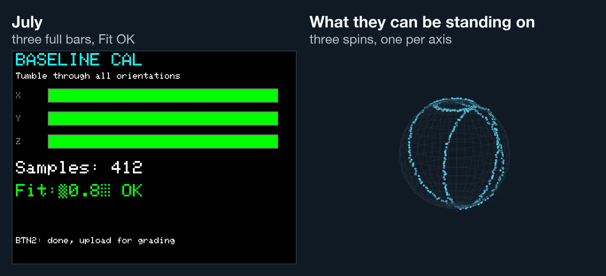
- The live fit number as a stop signal. Replayed against real runs, it settled on a steady value that was wrong, even when the data was good.
On July 26 I stopped pretending. The commit that retired the grid said it in six words: “collect honest, grade in the cloud.” The unit would show only what it could honestly know: a sample count and some rough bars, with no claim that you were done. It would also log the accelerometer and gyro alongside the compass, so that once a real fit existed, the server could work out after the fact which way each sample had been pointing.
The laptop goes away
The same week, calibration moved off the laptop. The unit links to a Dive Map account and uploads its samples over WiFi when a step finishes. The server runs the same fit code the laptop script did, and the result comes back to the unit’s own screen within about half a minute, with ACCEPT and REJECT. Every attempt goes into a calibration history on the website, accepted or not, and if a new calibration turns out worse, you can go back to an older one.
Getting rid of the laptop didn’t make the calibrations any better on its own. What it did was put the fit somewhere that could look at the data properly, and give me a place to see the answer.
What good calibration data actually is
With a real fit in hand, the server can do what no screen on the unit could at the time: look at a finished collection and say which orientations it has and hasn’t seen. Here’s a blind tumble from the day of my best full calibration run so far, graded the way the server grades every one now.
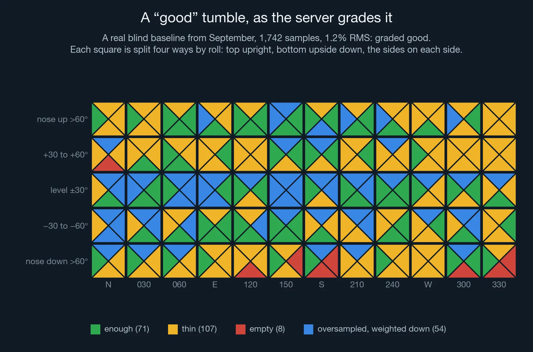
Of 240 orientation-and-roll cells, 71 were fine, 107 thin and 8 empty. Another 54 had so many samples that the server had to turn them down. Look at the pattern. The middle row, the unit held roughly level, is oversampled almost the whole way round, and the steep and upside-down cells are where the gaps are. That was a careful tumble by someone who’d been doing this for seven months.
Here’s what we now know good data needs:
| Needs | Why |
|---|---|
| Every orientation, including roll | An elevation-by-heading grid can read solid green while every sample in a box was taken right side up. Each box now tracks four roll positions, which is why the unit asks you to hold it upside down. |
| Balance | No orientation should outvote the others. More on this below. |
| Stillness, for the mounted step | The fit takes “down” from the accelerometer. A sample taken mid-swing has the wrong “down”, and one degree of false tilt leaks about 0.85 µT of the vertical field into the horizontal field the compass uses, about 5% of it. |
| Level, and a level reference, for the heading step | One rolled heading run looked like the unit was sensitive to roll. It was the reference compass tilting with the scooter. |
| The dive configuration | Same wiring, same desiccant, same temperature. If anything moves after you calibrate, you’ve calibrated a different object. |
The oversampling trap
This one caught us more than once.
A least-squares fit gives every sample one vote. Tumble the comfortable orientations for twice as long and they get twice the say. On its own that’s mostly harmless. When I piled 400 extra clean samples into one box of a real tumble, heading moved by a degree at most. The trouble starts when the oversampled spot is a little bit wrong. Then the fit bends the whole sphere toward it.
The clearest case came in July. Near the end of a baseline, I set the unit down to take a photo, right next to my desk speakers. 144 of that run’s 1,414 samples came from that one parked, magnetically disturbed spot, and they pushed the RMS from 2.76% to 5.20%. Quieter versions of the same thing kept turning up: a long pause at one orientation, a board still warming up, a few extra minutes in the level band because that’s where your hands want to be.
The fix has two halves.
Limits on the unit. During gap-fill, a targeted box stops accepting samples once it has enough: 15 right side up, and 5 in each other roll position. A box that isn’t a target takes only 4. During baseline, each box stops at twice its “finished” level, so the easy orientations can’t fill the 2,160-sample buffer before you’ve reached the hard ones. Even that took tuning. A limit of one times “finished” threw away 20–30% of the samples and bent the fit by up to 17° in the sparse orientations.
Normalization on the server. Each sample’s weight in the fit is divided by the number of samples that share its orientation, so every orientation gets roughly the same say however long you spent there. A floor stops a box with two stray samples from steering the whole fit the other way. On the desk-speakers run, measured against clean samples the fit never saw, the error dropped from 2.72% to 0.34%.
The grade had to change as well. Plain RMS averages over whatever you collected, so filling a gap could make the number worse: the new samples exposed error the old fit had never been tested against. Doing the right thing made the one number I was shown go the wrong way. The server now gives each orientation equal weight in the score, and compares an old and a new calibration on the same samples.
Telling the diver while they’re collecting
The rule we ended up with is simple: the screen only claims what the unit can honestly know at that moment.
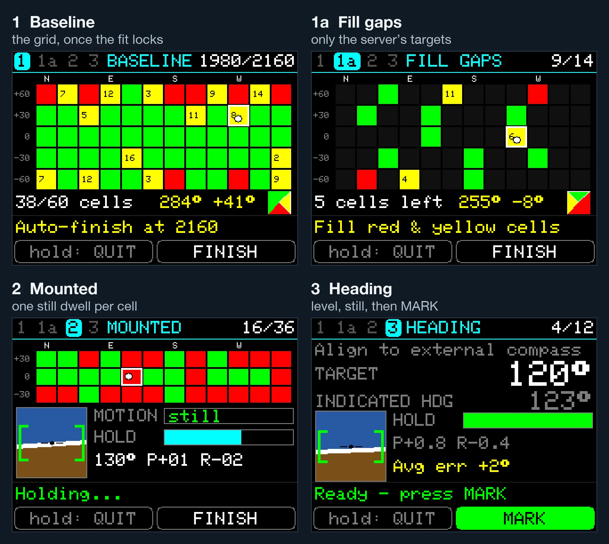
- Baseline starts with bars and no promises. Within the first 50 to 75 samples, a few seconds of tumbling, the unit fits a rough sphere of its own. Once that fit is stable, the grid appears, and each sample is placed with plain geometry from that fit, with no filter and no lag. Replayed against real runs, it puts 85–90% of samples in the same box the server would, and nearly all the rest one box over.
- Fill gaps asks only for the boxes the server flagged. A dot moves inside the grid ten times a second so you can steer toward a box, and the four-triangle widget shows which roll positions that box still needs. Full boxes stop accepting, so green means more there won’t help.
- Mounted fills one box per still moment. A box records only after the unit has sat still at the right attitude, and the motion and hold bars show how close you are.
- Heading lights MARK only when the unit is level within 3° and has been still for a second and a half. The target is the big number. The unit’s own reading is small and grey, so you line up with the compass instead of trying to make the two numbers match.
Getting here involved one more humbling bug. The first bench test of gap-fill was disorienting: nose up 45° pointing north lit the box for 30° nose-down, pointing south. Three sign errors in how the compass and accelerometer frames were combined. Two of them cancel exactly when the unit is level, which is why every test passed: the level-only axis test, dive logs that never tilt past 5°, and a 12,247-sample check that the Python and C++ versions agreed. They agreed perfectly, because both had the same bug. What finally caught it was a 13-pose physical fixture, the only test whose answer doesn’t come from the code. Turns out I’ve forgotten literally everything that Mrs. Sedgewick taught me about matrix math in the 9th grade.
The result screen got the same treatment.
Where it stands
Here’s the honest status.
The calibrations are now within the noise. On the bench, the final heading check lands within 1–2° at every point. That’s about as well as I can read the 2-inch compass on the scooter that I align everything against. In the water, what’s left over from dive to dive is about the size of what my GPS fixes can resolve. (Scoot to a point, ascend, get a fix — what’s the physical distance between where you stopped scooting and where you surfaced?) I can no longer measure the calibration’s error with the tools I’m checking it against.
The calibration is easy and intuitive. On-screen feedback actually tells you what to do next, and only collects data that’s beneficial to the calibration. You know while you’re collecting data that you’re getting it right. It no longer feels like black magic when I get a good cal — it feels like a brief chore, one more predictable checklist in the dive prep process.
That’s still mediocre. In real terms it’s ±2–3° on any given run. Over a 500 m leg, that’s 17–26 m off to one side. In Lake Washington, that’s still more than enough to miss the wreck. It’s not “different lake” bad, and it’s still much better than most of us can do by hand, but it’s not good enough to consistently hit a small target.
There are almost certainly errors I haven’t found yet. The two biggest surprises were temperature and magnetics that move, like a power wire that got pushed under the sensor after calibration. But I was just as surprised to find that what I lined the heading cal up against mattered. I’d been sighting along the nav tube, the housing the electronics live in. The thing that actually moves through the water is the scooter. Whatever small angle sits between the two went straight into the heading correction, where the 12-point check couldn’t see it, because the check used the same sighting. Now I align the scooter compass to the scooter tube, sighted against a distant object.
Who knows what I’ll learn next. Progress goes on the DPV-Nav project page.
What I’d tell past me
- “All directions” means the whole sphere. Upside down, on each side, nose straight down. Your hands will cover the level band twice and skip the bottom.
- A score that grades the samples you collected can’t see the ones you didn’t. RMS describes your data, not your coverage.
- Defining “good” is enormously important. If the user is collecting against a time limit, or against arbitrarily meaningless bars, they’re going to collect bad data. Define “good,” then grade against that during the collection.
- “OK” should mean right, not stable. A number that has stopped moving can still be wrong.
- Don’t let any orientation outvote the rest. Cap it while collecting, weight it while fitting.
- A screen should only claim what it can know right now. A confident grid fed a guessed heading is worse than a sample counter.
- Count the knobs. Nine numbers through twelve points will hit all twelve. Hold one out and see what the curve really knows.
- The reference is part of the calibration. That includes the compass you sight with, the tube you sight along, and whether either one is tilted.